The Kelly Criterion#
The Kelly Criterion determines the size of a bet in a repeated game with binary outcomes. The analysis was proposed in 1956 by John Kelly at Bell Laboratories. Kelly identified an analogy between gambling on binary outcomes and Claude Shannon’s work on encoding information for transmission on noisy channels. Kelly used the analogy to show
The maximum exponential rate of growth of the gambler’s capital is equal to the rate of transmission of information over the channel.
This idea actually predates Kelly. In 1738, Daniel Bernoulli offered a resolution to the St. Petersburg paradox proposed by his cousin, Nicholas Bernoulli. The resolution was to allocate bets among alternative outcomes to produce the highest geometric mean of returns. Kelly’s analysis has been popularized by William Poundstone in his book “Fortune’s Formula”, and picked up by gamblers with colorful adventures in Las Vegas by early adopters though the result laid in obscurity among investors until much later.
This notebook presents solutions to Kelly’s problem using exponential cones. A significant feature of this notebook is the inclusion of risk constraints recently proposed by Boyd and coworkers. These notes are based on recent papers by Busseti, Ryu, and Boyd (2016), Fu, Narasimhan, and Boyd (2017). Additional bibliographic notes are provided at the end of the notebook.
# install dependencies and select solver
%pip install -q amplpy numpy pandas

SOLVER_CONIC = "mosek"  # ipopt, mosek, knitro

from amplpy import AMPL, ampl_notebook

ampl = ampl_notebook(
    modules=["coin", "mosek"],  # modules to install
    license_uuid="default",  # license to use
)  # instantiate AMPL object and register notebook magics
import numpy as np
import pandas as pd
Optimal Log Growth#
The problem addressed by Kelly is to maximize the rate of growth of an investor’s wealth. At every stage \(n=1,\dots,N\), the gross return \(R_n\) on the investor’s wealth \(W_n\) is given by
After \(N\) stages, this gives
Kelly’s idea was to maximize the mean log return. Intuitively, this objective can be justified as we are simultaneously maximizing the geometric mean return
and the expected logarithmic utility of wealth
The logarithmic utility provides an element of risk aversion. If the returns \(R_i\)’s are independent and identically distributed random variables, then in the long run,
such that the optimal log growth return will almost surely result in higher wealth than any other policy.
Modeling a Game with Binary Outcomes#
The classical presentation of the Kelly Criterion is to consider repeated wagers on a gambling game with binary outcomes. For each stage, a wager of one unit returns \(1+b\) with probability \(p\) if successful, otherwise the wager returns nothing. The number \(b\) refers to the “odds” of game. The problem is to determine what fraction of the gambler’s wealth should be wagered on each instance of the game.
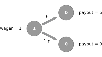
Let \(w\) be the fraction of wealth that is wagered on each instance. Depend on the two possible outcome, the gross return at any stage is
The objective is to the maximize the expected log return
The well-known analytical solution \(w^*\) to this problem can be calculated to be
We can use this analytical solution to validate the solution of this problem that we will now obtain using conic optimization.
Conic Optimization#
Recall that an exponential cone is a convex set \(\mathbf{K}_{\mathrm{exp}} \) of \(\mathbb{R}^3\) whose points \((r, x, y)\) satisfy the inequality
or the inequalities \(r \geq 0\) and \(y \leq 0\) if \(x=0\).
Introducing two auxiliary variables \(q_1\) and \(q_2\) and taking the exponential of the terms in the objective function, we obtain
and
With these constraints, Kelly’s problem becomes
The following code shows how to obtain an optimal solution using the AMPL conic optimization facilities and the Mosek solver.
%%writefile kelly.mod

# parameter values
param b;
param p;

# decision variables
var q1;
var q2;
var w >= 0;

# objective
maximize ElogR:
    p*q1 + (1-p)*q2;

# conic constraints
s.t. T1: 1 + b*w >= exp( q1 );
s.t. T2: 1 - w   >= exp( q2 );
Overwriting kelly.mod
# parameter values
b = 1.25
p = 0.51


# conic optimization solution to Kelly's problem
def kelly(p, b):
    # Create AMPL instance and load the model
    ampl = AMPL()
    ampl.read("kelly.mod")

    # load the data
    ampl.param["b"] = b
    ampl.param["p"] = p

    # solve
    ampl.option["solver"] = SOLVER_CONIC
    ampl.solve()

    return ampl.get_value("w")


w_conic = kelly(p, b)
print(f"Conic optimization solution for w: {w_conic: 0.4f}")

# analytical solution to Kelly's problem
w_analytical = p - (1 - p) / b if p * (b + 1) > 1 else 0
print(f"Analytical solution for w: {w_analytical: 0.4f}")
MOSEK 10.0.43: MOSEK 10.0.43: optimal; objective 0.008642708771
0 simplex iterations
8 barrier iterations
Conic optimization solution for w:  0.1180
Analytical solution for w:  0.1180
Risk-constrained version of the Kelly’s problem#
Following Busseti, Ryu, and Boyd (2016), we consider the risk-constrained version of the Kelly’s problem, in which we add the constraint
where \(\lambda \geq 0\) is a risk-aversion parameter. For the case with two outcomes \(R_1\) and \(R_2\) with known probabilities \(p_1\) and \(p_2\) considered here, this constraint rewrites as
When \(\lambda=0\) the constraint is always satisfied and no risk-aversion is in effect. Choosing \(\lambda > 0\) requires outcomes with low return to occur with low probability and this effect increases for larger values of \(\lambda\). A feasible solution can always be found by setting the bet size \(w=0\) to give \(R_1 = 1\) and \(R_2 = 0\).
This constraint can be reformulated using exponential cones. Rewriting each term as an exponential results gives
We previously introduced two auxiliary real variables \(q_1,q_2 \in \mathbb{R}\) such that \(q_i \leq \log(R_i)\), using which we can reformulate the risk constraint as
Introducing two more non-negative auxiliary variables \(u_1,u_2 \geq 0\) such that \(u_i \geq e^{\log(p_i) - \lambda q_i}\), the risk constraint is given by
For fixed probabilities \(p_1=p\) and \(p_2=1-p\), odds \(b\), and risk-aversion parameter \(\lambda \geq 0\), the risk-constrained Kelly bet is a solution to the conic optimization problem rewrites as
The following cell solves this problem with an AMPL model using the Mosek solver.
%%writefile kelly_rc.mod

# parameter values
param b;
param p;
param lambd;

# decision variables
var q1;
var q2;
var w >= 0;

# objective
maximize ElogR:
    p*q1 + (1-p)*q2;

# conic constraints
s.t. T1: 1 + b*w >= exp( q1 );
s.t. T2: 1 - w   >= exp( q2 );

# risk constraints
var u1 >= 0;
var u2 >= 0;
s.t. R0: u1 + u2 <= 1;
s.t. R1: u1 >= exp(log(p) - lambd*q1);
s.t. R2: u2 >= exp(log(1 - p) - lambd*q2);
Overwriting kelly_rc.mod
import numpy as np

# parameter values
b = 1.25
p = 0.51
lambd = 3


# conic optimization solution to Kelly's problem
def kelly_rc(p, b, lambd):
    # Create AMPL instance and load the model
    ampl = AMPL()
    ampl.read("kelly_rc.mod")

    # load the data
    ampl.param["b"] = b
    ampl.param["p"] = p
    ampl.param["lambd"] = lambd

    # solve
    ampl.option["solver"] = SOLVER_CONIC
    ampl.solve()

    return ampl.get_value("w")


w_rc = kelly_rc(p, b, lambd)
print(f"Risk-constrainend solution for w: {w_rc: 0.4f}")

# solution to Kelly's problem
w_analytical = p - (1 - p) / b if p * (b + 1) >= 1 else 0
print(f"Analytical solution for w: {w_analytical: 0.4f}")
MOSEK 10.0.43: MOSEK 10.0.43: optimal; objective 0.006486710424
0 simplex iterations
9 barrier iterations
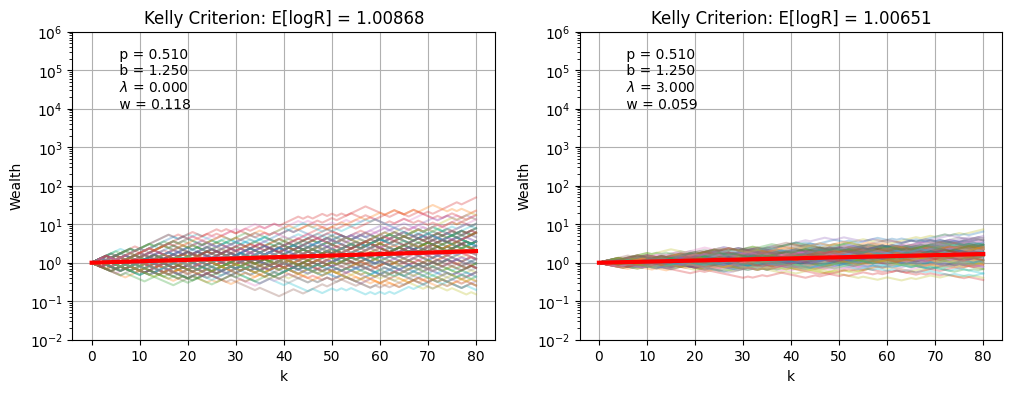
Risk-constrainend solution for w: 0.0589
Analytical solution for w: 0.1180
Simulation#
The following cells simulate the performance of the Kelly Criterion both with and without risk constraints. Compare the cases by comparing the log mean growth, which is reduced by presence of risk constraints, and the portfolio draw down for the most pathological cases, which is improved by the presence of risk constraints.
import numpy as np
import matplotlib.pyplot as plt


def kelly_sim(p, b, lambd=0, K=None, ax=None):
    w = kelly_rc(p, b, lambd)
    m = p * np.log((1 + b * w)) + (1 - p) * np.log((1 - w))

    if K is None:
        K = int(np.log(10) / m)
    if ax is None:
        _, ax = plt.subplots(1, 1)

    # monte carlo simulation and plotting
    for n in range(0, 100):
        W = [1]
        R = [[1 - w, 1 + w * b][z] for z in np.random.binomial(1, p, size=K)]
        R.insert(0, 1)
        ax.semilogy(np.cumprod(R), alpha=0.3)

    ax.semilogy(np.linspace(0, K), np.exp(m * np.linspace(0, K)), "r", lw=3)
    ax.set_title(f"Kelly Criterion: E[logR] = {np.exp(m):0.5f}")
    s = f" p = {p:0.3f} \n b = {b:0.3f} \n $\lambda$ = {lambd:0.3f} \n w = {w:0.3f}"
    ax.text(0.1, 0.95, s, transform=ax.transAxes, va="top")
    ax.set_xlabel("k")
    ax.set_ylabel("Wealth")
    ax.grid(True)
    ax.set_ylim(0.01, 1e6)


fig, ax = plt.subplots(1, 2, figsize=(12, 4))

kelly_sim(p, b, lambd=0, K=80, ax=ax[0])
kelly_sim(p, b, lambd=3, K=80, ax=ax[1])
MOSEK 10.0.43: MOSEK 10.0.43: optimal; objective 0.008642708771
0 simplex iterations
8 barrier iterations
MOSEK 10.0.43: MOSEK 10.0.43: optimal; objective 0.006486710424
0 simplex iterations
9 barrier iterations
Bibliographic Notes#
The Kelly Criterion has been included in many tutorial introductions to finance and probability, and the subject of popular accounts.
Poundstone, W. (2010). Fortune’s formula: The untold story of the scientific betting system that beat the casinos and Wall Street. Hill and Wang. https://www.onlinecasinoground.nl/wp-content/uploads/2020/10/Fortunes-Formula-boek-van-William-Poundstone-oa-Kelly-Criterion.pdf
Thorp, E. O. (2017). A man for all markets: From Las Vegas to wall street, how i beat the dealer and the market. Random House.
Thorp, E. O. (2008). The Kelly criterion in blackjack sports betting, and the stock market. In Handbook of asset and liability management (pp. 385-428). North-Holland. https://www.palmislandtraders.com/econ136/thorpe_kelly_crit.pdf
The utility of conic optimization to solve problems involving log growth is more recent. Here are some representative papers.
Busseti, E., Ryu, E. K., & Boyd, S. (2016). Risk-constrained Kelly gambling. The Journal of Investing, 25(3), 118-134. https://arxiv.org/pdf/1603.06183.pdf
Fu, A., Narasimhan, B., & Boyd, S. (2017). CVXR: An R package for disciplined convex optimization. arXiv preprint arXiv:1711.07582. https://arxiv.org/abs/1711.07582