Economic Order Quantity#
This notebook demonstrates the reformulation of hyperbolic constraints as standard SOCO and also the direct modeling of the hyperbolic constraint. The example is familiar to any MBA/business student, and has a significant range of applications including warehouse operations.
Usage notes#
The notebook requires a solver that can handle conic constraints. AMPL provides interfaces to the commercial solvers Gurobi and Mosek that include conic solvers. Other nonlinear solvers may solve these problems using more general techniques that are not specific to conic constraints.
Free licenses are available for academic use of
mosekandgurobi.If you do not have access to Gurobi or Mosek, you can use the
ipoptsolver. Note, however, thatipoptis a general purpose interior point solver, and does not have algorithms specific to conic problems.
# install dependencies and select solver
%pip install -q amplpy numpy pandas

SOLVER_CONIC = "mosek"  # ipopt, mosek, gurobi, knitro

from amplpy import AMPL, ampl_notebook

ampl = ampl_notebook(
    modules=["coin", "mosek"],  # modules to install. ipopt is part of coin
    license_uuid="default",  # license to use
)  # instantiate AMPL object and register notebook magics
import numpy as np
import pandas as pd
Please provide a valid license UUID. You can use a free https://ampl.com/ce license.
The EOQ model#
Classical formulation for a single item#
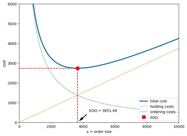
The economic order quantity (EOQ) is a classical problem in inventory management attributed to Ford Harris (1915). The problem is to find the order quantity that minimizes the cost of maintaining a specific item in inventory
The cost for maintaining an item in inventory given an order size \(x\) is given by
where \(h\) is the annual cost of holding an item including financing charges, \(c\) is the fixed cost of placing and receiving an order, and \(d\) is the annual demand. The factor \(\frac{1}{2}\) is a result of demand depletes the inventory at a constant rate over the year. The economic order quantity is the value of \(x\) that minimizes \(f(x)\)
Given the rather simple domain, we can derive analytically the solution for the EOQ problem by setting the derivative of \(f(x)\) equal to zero and solving the resulting equation, obtaining
The following chart illustrates the nature of the problem and its analytical solution.
import matplotlib.pyplot as plt
import numpy as np

h = 0.75  # cost of holding one item for one year
c = 500.0  # cost of processing one order
d = 10000.0  # annual demand

eoq = np.sqrt(2 * c * d / h)
fopt = np.sqrt(2 * c * d * h)
print(f"Optimal order size = {eoq:0.1f} items with cost {fopt:0.2f}")

x = np.linspace(100, 10000, 1000)
f = h * x / 2 + c * d / x

fig, ax = plt.subplots(figsize=(8, 6))
ax.plot(x, f, lw=3, label="total cost")
ax.plot(x, h * x / 2, "--", lw=1, label="holding costs")
ax.plot(x, c * d / x, "--", lw=1, label="ordering costs")
ax.set_xlabel("x = order size")
ax.set_ylabel("cost")
ax.plot(eoq, fopt, "ro", ms=10, label="EOQ")
ax.legend(loc="lower right")
ax.annotate(
    f"EOQ = {eoq:0.2f}",
    xy=(eoq, 0),
    xytext=(1.2 * eoq, 0.2 * fopt),
    arrowprops=dict(facecolor="black", shrink=0.15, width=1, headwidth=6),
)
ax.plot([eoq, eoq, 0], [0, fopt, fopt], "r--")
ax.set_xlim(0, 10000)
ax.set_ylim(0, 6000);
Optimal order size = 3651.5 items with cost 2738.61
Reformulating EOQ as a linear objective with hyperbolic constraint#
However, if the problem involved multiple products, an analytical solution would no longer be easily available. For this reason, we need to be able to solve the problem numerically, let us see how.
It can be easily checked that the objective \(f(x)\) is a convex function and therefore, the problem can be solved using any convex optimization solver. It is, however, a special type of convex problem which we shall show in the following reformulation.
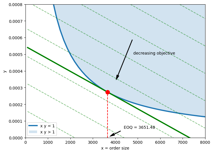
The optimization objective is linearized with the use of a second decision variable \(y = 1/x\). The optimization problem is now a linear objective in two decision variables with a hyperbolic constraint \(xy \geq 1\).
This constraint and the linear contours of the objective function are shown in the following diagrams. The solution of optimization problem occurs at a point where the constraint is tangent to contours of the objective function.
import matplotlib.pyplot as plt
import numpy as np

h = 0.75  # cost of holding one item for one year
c = 500.0  # cost of processing one order
d = 10000.0  # annual demand

x = np.linspace(100, 8000)
y = (fopt - h * x / 2) / (c * d)

eoq = np.sqrt(2 * c * d / h)
fopt = np.sqrt(2 * c * d * h)
yopt = (fopt - h * eoq / 2) / (c * d)

fig, ax = plt.subplots(figsize=(8, 6))
ax.plot(x, 1 / x, lw=3, label="x y = 1")
ax.plot(x, (fopt - h * x / 2) / (c * d), "g", lw=3)
for f in fopt * np.linspace(0, 3, 11):
    ax.plot(x, (f - h * x / 2) / (c * d), "g--", alpha=0.5)
ax.plot(eoq, yopt, "ro", ms=10)
ax.annotate(
    f"EOQ = {eoq:0.2f}",
    xy=(eoq, 0),
    xytext=(1.2 * eoq, 0.2 * yopt),
    arrowprops=dict(facecolor="black", shrink=0.15, width=1, headwidth=6),
)

ax.annotate(
    "",
    xytext=(4800, 0.0006),
    xy=(4000, 1 / 3000),
    arrowprops=dict(facecolor="black", shrink=0.05, width=1, headwidth=6),
)
ax.text(4800, 0.0005, "decreasing objective")
ax.fill_between(x, 1 / x, 0.0008, alpha=0.2, label="x y > 1")
ax.plot([eoq, eoq], [0, yopt], "r--")

ax.set_xlim(0, 8000)
ax.set_ylim(0, 0.0008)
ax.set_xlabel("x = order size")
ax.set_ylabel("y")
ax.legend();
Reformulating the EOQ model with a linear objective and a second order cone constraint#
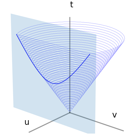
In elementary geometry, a hyperbola can be constructed from the intersection of a linear plane with cone. For this application, the hyperbola described by the constraint \(x y \geq 1\) invites the question of whether there is reformulation of EOQ that includes a cone constraint.
A Lorenz cone is defined by
where the components of are given by \(z = \begin{bmatrix} u \\ v \end{bmatrix}\). The intersection of a plane aligned with the \(t\) axis exactly describes a hyperbola. As described by Lobo, et al. (1998), the correspondence is given by
where the axis in the \(w, x, y\) coordinates is tilted, displaced, and stretched compared to the coordinates shown in the diagram. The exact correspondence to the diagram is given by
The Python code below draws a hyperbola precisely as the intersection of a plane with Lorenz cone.
Let us know rewrite the nonlinear constraint of the EOQ problem. Using the same geometric idea as above and leveraging the non-negativity of both variables, the constraint \(xy \geq 1\) can be reformulated using the following trick:
where we rely on the fact that \(x + y \geq 0\). The final constraint is known as a second-order conic optimization constraint (SOCO constraint). The result is a reformulation of the EOQ problem as a second order conic optimization (SOCO).
import matplotlib.pyplot as plt
import numpy as np
from mpl_toolkits import mplot3d
import mpl_toolkits.mplot3d.art3d as art3d
from matplotlib.patches import Rectangle

t_max = 4
w = 2
n = 40

fig = plt.figure(figsize=(9, 7))
ax = plt.axes(projection="3d")

for t in np.linspace(0, t_max, n + 1):
    if t < w:
        a = np.linspace(0, 2 * np.pi, 30)
        u = t * np.cos(a)
        v = t * np.sin(a)
        ax.plot3D(u, v, t, "b", lw=0.3)
    else:
        b = np.arccos(w / t)
        a = np.linspace(b, 2 * np.pi - b, 30)
        u = t * np.cos(a)
        v = t * np.sin(a)
        ax.plot3D(u, v, t, "b", lw=0.3)
        ax.plot3D([2, 2], [t * np.sin(b), -t * np.sin(b)], [t, t], "b", lw=0.3)

t = np.linspace(w, t_max)
v = t * np.sin(np.arccos(w / t))
u = w * np.array([1] * len(t))
ax.plot3D(u, v, t, "b")
ax.plot3D(u, -v, t, "b")

ax.plot3D([0, t_max + 0.5], [0, 0], [0, 0], "k", lw=3, alpha=0.4)
ax.plot3D([0, 0], [0, t_max + 1], [0, 0], "k", lw=3, alpha=0.4)
ax.plot3D([0, 0], [0, 0], [0, t_max + 1], "k", lw=3, alpha=0.4)

ax.text3D(t_max + 1, 0, 0.5, "u", fontsize=24)
ax.text3D(0, t_max, 0.5, "v", fontsize=24)
ax.text3D(0, 0, t_max + 1.5, "t", fontsize=24)

ax.view_init(elev=20, azim=40)

r = Rectangle((-t_max, 0), 2 * t_max, t_max + 1, alpha=0.2)
ax.add_patch(r)
art3d.pathpatch_2d_to_3d(r, z=w, zdir="x")

ax.grid(False)
ax.axis("off")

ax.set_xlabel("u")
ax.set_ylabel("v")

ax.set_xlim(-3, 3)
ax.set_ylim(-3, 3)
ax.set_zlim(1, 4)
plt.show()
AMPL modeling of second-order cones#
The SOCO formulation given above needs to be reformulated one more time into one of the standard forms:
where the \(x_i\) and \(r\) terms are AMPL variables. The first step is to introduce rotated coordinates \(t = x+ y\) and \(v = x - y\), and (optionally) introduce a new variable with fixed value \(u = 2\),
This version of the model with variables \(t, u, v, x, y\) could be implemented directly in AMPL. However, the model can be further reduced to yield a simpler version of the model.
The EOQ model is now ready to implement. AMPL provides drivers for the Mosek and Gurobi commercial solvers (note that academic licenses are available at no cost). These drivers recognize the SOCO constraints and pass them to the solvers.
%%writefile eoq_soc_basic.mod

param h;      # cost of holding one item for one year
param c;      # cost of processing one order
param d;      # annual demand

# define variables for conic constraints
var u >= 0;
var v >= 0;
var t >= 0;

# relationships for conic constraints to decision variables
s.t. u_eq:
    u == 2;

# conic constraint
s.t. q:
    t^2 >= u^2 + v^2;

# linear objective
minimize eoq:
    ((h + 2*c*d)*t + (h - 2*c*d)*v)/4;
Overwriting eoq_soc_basic.mod
h = 0.75  # cost of holding one item for one year
c = 500.0  # cost of processing one order
d = 10000.0  # annual demand

# Create AMPL instance and load the model
ampl = AMPL()
ampl.read("eoq_soc_basic.mod")

# load the data
ampl.param["h"] = h
ampl.param["c"] = c
ampl.param["d"] = d

# solve
ampl.option["solver"] = SOLVER_CONIC
ampl.solve()


# solution
print(f"\nEOQ = { ampl.get_value('(t + v)/2') :.2f}")
MOSEK 10.0.43: MOSEK 10.0.43: unknown (0, problem status: 0), stalling
0 simplex iterations
15 barrier iterations

EOQ = 3653.04
Another standard SOCO representation#
AMPL conic solvers allow the alternative SOCO representation according to the definition of a Lorenz cone:
Moreover here we go all the way and don’t use the auxiliary variable u fixed to a constant value. The required value can simply be inserted directly into constraint specification as demonstrated below.
%%writefile eoq_soc.mod

param h;      # cost of holding one item for one year
param c;      # cost of processing one order
param d;      # annual demand

# define variables for conic constraints
var v >= 0;
var t >= 0;

# conic constraint
s.t. q:
    -t <= -sqrt(2^2 + v^2);

# linear objective
minimize eoq:
    ((h + 2*c*d)*t + (h - 2*c*d)*v)/4;
Overwriting eoq_soc.mod
h = 0.75  # cost of holding one item for one year
c = 500.0  # cost of processing one order
d = 10000.0  # annual demand

# Create AMPL instance and load the model
ampl = AMPL()
ampl.read("eoq_soc.mod")

# load the data
ampl.param["h"] = h
ampl.param["c"] = c
ampl.param["d"] = d

# solve
ampl.option["solver"] = SOLVER_CONIC
ampl.solve()


# solution
print(f"\nEOQ = { ampl.get_value('(t + v)/2') :.2f}")
MOSEK 10.0.43: MOSEK 10.0.43: unknown (0, problem status: 0), stalling
0 simplex iterations
15 barrier iterations

EOQ = 3653.04
AMPL modeling with rotated second-order cones#
The need to rotate the natural coordinates of the EOQ problem to fit the programming interface to standard cones is not a big stumbling block, but does raise the question of whether there is a more natural way to express hyperbolic or cone constraints in AMPL.
Rotated second-order cones have the form
This enables a direct expression of the hyperbolic constraint \(x y \geq 1\) by introducing an optional auxiliary variable \(z\) with fixed value \(z^2 = 2\), such that
The model to be implemented in AMPL is now
However the trick with the auxilary variable \(z\) is optional and omitted in the implementation below, substituting the constant value \(\sqrt2\) directly. Note the improvement in accuracy of this calculation, compared to the previous solutions.
%%writefile eoq_rsoc.mod

param h;      # cost of holding one item for one year
param c;      # cost of processing one order
param d;      # annual demand

# define variables for conic constraints
var x >= 0;
var y >= 0;

# conic constraint
s.t. q:
    x*y >= 1;

# linear objective
minimize eoq:
    h*x/2 + c*d*y;
Overwriting eoq_rsoc.mod
h = 0.75  # cost of holding one item for one year
c = 500.0  # cost of processing one order
d = 10000.0  # annual demand

# Create AMPL instance and load the model
ampl = AMPL()
ampl.read("eoq_rsoc.mod")

# load the data
ampl.param["h"] = h
ampl.param["c"] = c
ampl.param["d"] = d

# solve
ampl.option["solver"] = SOLVER_CONIC
ampl.solve()


# solution
print(f"\nEOQ = { ampl.get_value('x') :.2f}")
MOSEK 10.0.43: MOSEK 10.0.43: optimal; objective 2738.612791
0 simplex iterations
10 barrier iterations

EOQ = 3651.46
Extending the EOQ model to multiple items with a shared resource#
Solving for the EOQ for a single item using SOCO optimization is using a sledgehammer to swat a fly. However, the problem becomes more interesting for determining economic order quantities when the inventories for multiple items compete for a shared resource in a common warehouse. The shared resource could be the financing available to hold inventory, space in a warehouse, or specialized facilities to hold a perishable good:
where \(h_i\) is the annual holding cost for one unit of item \(i\), \(c_i\) is the cost to place an order and receive delivery for item \(i\), and \(d_i\) is the annual demand. The additional constraint models an allocation of \(b_i\) units of the shared resource, and \(b_0\) is the total resource available.
Following the reformulation of the single item model, a variable \(y_i \geq 0\), \(i=1, \dots, n\) is introduced to linearize the objective
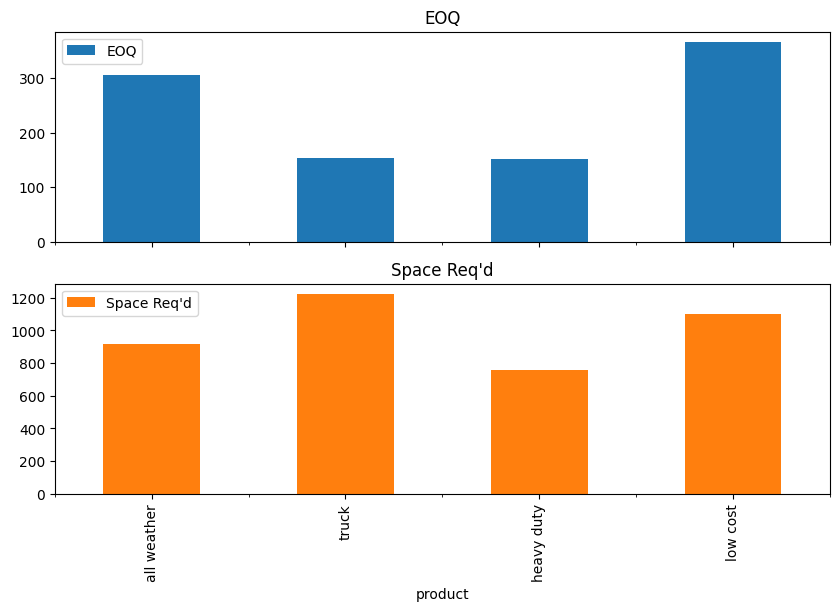
The following AMPL model is a direct implementation of the multi-item EOQ formulation and applied to a hypothetical car parts store that maintains an inventory of tires.
import pandas as pd

df = pd.DataFrame(
    {
        "all weather": {"h": 1.0, "c": 200, "d": 1300, "b": 3},
        "truck": {"h": 2.8, "c": 250, "d": 700, "b": 8},
        "heavy duty": {"h": 1.2, "c": 200, "d": 500, "b": 5},
        "low cost": {"h": 0.8, "c": 180, "d": 2000, "b": 3},
    }
).T

display(df)
| h | c | d | b | |
|---|---|---|---|---|
| all weather | 1.0 | 200.0 | 1300.0 | 3.0 |
| truck | 2.8 | 250.0 | 700.0 | 8.0 |
| heavy duty | 1.2 | 200.0 | 500.0 | 5.0 |
| low cost | 0.8 | 180.0 | 2000.0 | 3.0 |
%%writefile eoq_multi_rsoc.mod

set ITEMS;

param b0;            # resource total
param b{ITEMS};      # resource per unit of each item
param h{ITEMS};      # cost of holding each item for one year
param c{ITEMS};      # cost of processing one order
param d{ITEMS};      # annual demand of each item

# define variables for conic constraints
var x {ITEMS} >= 0;
var y {ITEMS} >= 0;

# conic constraints
s.t. q {i in ITEMS}:
    x[i]*y[i] >= 1;

# resource capacity
s.t. r:
    sum {i in ITEMS} (b[i]*x[i]) <= b0;

# linear objective
minimize eoq:
    sum {i in ITEMS}
        (h[i]*x[i]/2 + c[i]*d[i]*y[i]);
Overwriting eoq_multi_rsoc.mod
import numpy as np

display(df)


def eoq(df, b):
    # Create AMPL instance and load the model
    ampl = AMPL()
    ampl.read("eoq_multi_rsoc.mod")

    # load the data
    ampl.set["ITEMS"] = list(df.index)
    ampl.set_data(df, "ITEMS")

    ampl.param["b0"] = b

    # solve
    ampl.option["solver"] = SOLVER_CONIC
    ampl.solve()

    return ampl


def eoq_display_results(df, ampl):
    x = ampl.get_variable("x")
    dfx = x.to_dict()

    results = pd.DataFrame(
        [[i, dfx[i], dfx[i] * df.loc[i, "b"]] for i in df.index],
        columns=["product", "EOQ", "Space Req'd"],
    ).round(1)
    results.set_index("product", inplace=True)

    display(results)
    results.plot(
        y=["EOQ", "Space Req'd"],
        kind="bar",
        subplots=True,
        layout=(2, 1),
        figsize=(10, 6),
    )


m = eoq(df, 4000)
eoq_display_results(df, m)
| h | c | d | b | |
|---|---|---|---|---|
| all weather | 1.0 | 200.0 | 1300.0 | 3.0 |
| truck | 2.8 | 250.0 | 700.0 | 8.0 |
| heavy duty | 1.2 | 200.0 | 500.0 | 5.0 |
| low cost | 0.8 | 180.0 | 2000.0 | 3.0 |
MOSEK 10.0.43: MOSEK 10.0.43: optimal; objective 4239.725348
0 simplex iterations
16 barrier iterations
| EOQ | Space Req'd | |
|---|---|---|
| product | ||
| all weather | 306.2 | 918.7 |
| truck | 153.2 | 1225.3 |
| heavy duty | 151.0 | 754.9 |
| low cost | 367.0 | 1101.1 |
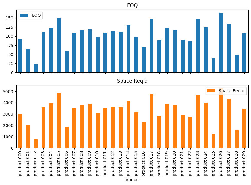
Testing the model on larger problems#
The following cell creates a random EOQ problem of size \(n\) that can be used to test the model formulation and solver.
n = 30

df_large = pd.DataFrame()
df_large["h"] = np.random.uniform(0.5, 2.0, n)
df_large["c"] = np.random.randint(300, 500, n)
df_large["d"] = np.random.randint(100, 5000, n)
df_large["b"] = np.random.uniform(10, 50)
df_large.set_index(pd.Series(f"product {i:03d}" for i in range(n)), inplace=True)

df_large

m = eoq(df_large, 100000)
eoq_display_results(df_large, m)
MOSEK 10.0.43: MOSEK 10.0.43: optimal; objective 252756.6403
0 simplex iterations
16 barrier iterations
| EOQ | Space Req'd | |
|---|---|---|
| product | ||
| product 000 | 92.1 | 2958.3 |
| product 001 | 64.6 | 2075.1 |
| product 002 | 23.1 | 742.9 |
| product 003 | 110.9 | 3562.1 |
| product 004 | 123.1 | 3952.4 |
| product 005 | 150.4 | 4830.2 |
| product 006 | 58.8 | 1886.9 |
| product 007 | 109.6 | 3518.3 |
| product 008 | 116.8 | 3751.3 |
| product 009 | 119.0 | 3823.2 |
| product 010 | 96.8 | 3107.7 |
| product 011 | 109.6 | 3519.6 |
| product 012 | 112.8 | 3623.5 |
| product 013 | 110.9 | 3562.2 |
| product 014 | 129.5 | 4160.2 |
| product 015 | 98.1 | 3152.0 |
| product 016 | 69.8 | 2243.2 |
| product 017 | 148.0 | 4752.9 |
| product 018 | 88.3 | 2834.6 |
| product 019 | 121.6 | 3905.3 |
| product 020 | 117.3 | 3765.9 |
| product 021 | 90.8 | 2916.2 |
| product 022 | 86.0 | 2763.0 |
| product 023 | 146.5 | 4703.9 |
| product 024 | 124.3 | 3991.4 |
| product 025 | 38.9 | 1250.4 |
| product 026 | 164.5 | 5282.0 |
| product 027 | 134.3 | 4311.7 |
| product 028 | 49.1 | 1576.4 |
| product 029 | 108.3 | 3477.0 |
Bibliographic notes#
The original formulation and solution of the economic order quantity problem is attributed to Ford Harris, but in a curious twist has been cited incorrectly since 1931. The correct citation is:
Harris, F. W. (1915). Operations and Cost (Factory Management Series). A. W. Shaw Company, Chap IV, pp.48-52. Chicago.
Harris later developed an extensive consulting business and the concept has become embedded in business practice for over 100 years. Harris’s single item model was later extended to multiple items sharing a resource constraint. There may be earlier citations, but this model is generally attributed to Ziegler (1982):
Ziegler, H. (1982). Solving certain singly constrained convex optimization problems in production planning. Operations Research Letters, 1(6), 246-252. https://www.sciencedirect.com/science/article/abs/pii/016763778290030X
Bretthauer, K. M., & Shetty, B. (1995). The nonlinear resource allocation problem. Operations research, 43(4), 670-683. https://www.jstor.org/stable/171693?seq=1
Reformulation of the multi-item EOQ model as a conic optimization problem is attributed to Kuo and Mittleman (2004) using techniques described by Lobo, et al. (1998):
Kuo, Y. J., & Mittelmann, H. D. (2004). Interior point methods for second-order cone programming and OR applications. Computational Optimization and Applications, 28(3), 255-285. https://link.springer.com/content/pdf/10.1023/B:COAP.0000033964.95511.23.pdf
Lobo, M. S., Vandenberghe, L., Boyd, S., & Lebret, H. (1998). Applications of second-order cone programming. Linear algebra and its applications, 284(1-3), 193-228. https://web.stanford.edu/~boyd/papers/pdf/socp.pdf
The multi-item model has been used didactically many times since 2004. These are representative examples
Letchford, A. N., & Parkes, A. J. (2018). A guide to conic optimisation and its applications. RAIRO-Operations Research, 52(4-5), 1087-1106. http://www.cs.nott.ac.uk/~pszajp/pubs/conic-guide.pdf
El Ghaoui, Laurent (2018). Lecture notes on Optimization Models. https://inst.eecs.berkeley.edu/~ee127/fa19/Lectures/12_socp.pdf
Mosek Modeling Cookbook, section 3.3.5. https://docs.mosek.com/modeling-cookbook/cqo.html.
Appendix: Formulation with SOCO constraints#
AMPL’s facility for direct handling of hyperbolic constraints bypasses the need to formulate SOCO constraints for the multi-item model. For completeness, however, that development is included here.
As a short cut to reformulating the model with conic constraints, note that a “completion of square” gives the needed substitutions
The multi-item EOQ model is now written with conic constraints
Variables \(t_i\), \(u_i\), and \(v_i\) are introduced t complete the reformulation for implementation with AMPL/Mosek.