Ordinary Least Squares (OLS) Regression

In Chapter 2 we introduced linear regression with least absolute deviations (LAD), see this notebook. Here we consider the same problem setting, but slightly change the underlying optimization problem, in particular its objective function, obtaining the classical ordinary least squares (OLS) regression.

# install AMPL and solvers
%pip install -q amplpy

SOLVER_LO = "cbc"
SOLVER_QO = "ipopt"

from amplpy import AMPL, ampl_notebook

ampl = ampl_notebook(
    modules=["coin"],  # modules to install
    license_uuid="default",  # license to use
)  # instantiate AMPL object and register magics

     ━━━━━━━━━━━━━━━━━━━━━━━━━━━━━━━━━━━━━━━━ 4.4/4.4 MB 13.8 MB/s eta 0:00:00
?25hUsing default Community Edition License for Colab. Get yours at: https://ampl.com/ce
Licensed to AMPL Community Edition License for the AMPL Model Colaboratory (https://colab.ampl.com).

Generate data

The Python scikit learn library for machine learning provides a full-featured collection of tools for regression. The following cell uses make_regression from scikit learn to generate a synthetic data set for use in subsequent cells. The data consists of a numpy array y containing n_samples of one dependent variable \(y\), and an array X containing n_samples observations of n_features independent explanatory variables.

from sklearn.datasets import make_regression
import numpy as np
import matplotlib.pyplot as plt

n_features = 1
n_samples = 500
noise = 75

# generate regression dataset
np.random.seed(2022)
X, y = make_regression(n_samples=n_samples, n_features=n_features, noise=noise)

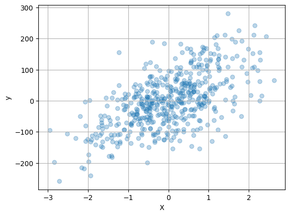
Data Visualization

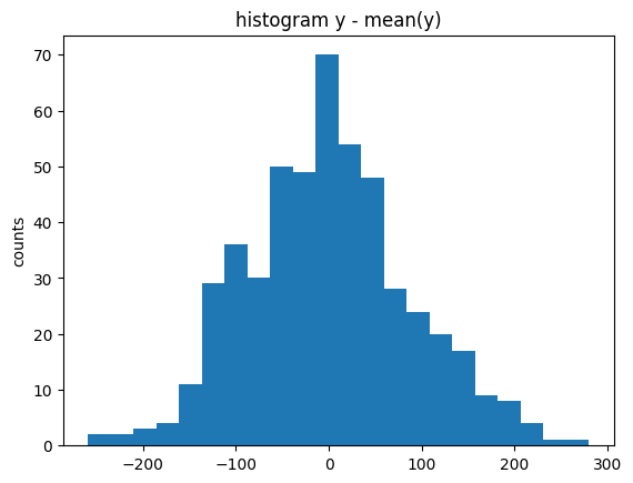
Before going further, it is generally useful to prepare an initial visualization of the data. The following cell presents a scatter plot of \(y\) versus \(x\) for the special case of one explanatory variable, and a histogram of the difference between \(y\) and the mean value \(\bar{y}\). This histogram will provide a reference against which to compare the residual error in \(y\) after regression.

if n_features == 1:
    plt.scatter(X, y, alpha=0.3)
    plt.xlabel("X")
    plt.ylabel("y")
    plt.grid(True)

plt.figure()
plt.hist(y - np.mean(y), bins=int(np.sqrt(len(y))))
plt.title("histogram y - mean(y)")
plt.ylabel("counts")
plt.show()

Model

Similarly to the LAD regression example, suppose we have a finite data set consisting of \(n\) points \(\{({X}^{(i)}, y^{(i)})\}_{i=1,\dots,n}\) with \({X}^{(i)} \in \mathbb R^k\) and \(y^{(i)} \in \mathbb R\). We want to fit a linear model with intercept, whose error or deviation term \(e_i\) is equal to

\[ e_i = y^{(i)} - {m}^\top {X}^{(i)} - b = y^{(i)} - \sum_{j=1}^k X^{(i)}_j m_j - b, \]

for some real numbers \(b, m_1,\dots,m_k\). The Ordinary Least Squares (OLS) is a possible statistical optimality criterion for such a linear regression, which tries to minimize the sum of the errors squares, that is \(\sum_{i=1}^n e_i^2\). The OLS regression can thus be formulated as an optimization with the coefficients \(b\) and \(m_i\)’s and the errors \(e_i\)’s as the decision variables, namely

\[\begin{split} \begin{align} \min \quad & \sum_{i=1}^n e_i^2\\ \text{s.t.} \quad & e_i = y^{(i)} - {m}^\top {X}^{(i)} - b, \qquad \forall\, i=1,\dots,n. \end{align} \end{split}\]

def ols_regression(X, y):
    m = AMPL()
    m.eval(
        """
      reset;

      set I;
      set J;
      
      var e{I};
      var m{J};
      var b;

      param X{I, J};
      param y{I};

      subject to residuals{i in I}:
        e[i] = y[i] - sum{j in J} X[i,j]*m[j] - b;

      minimize sum_of_square_errors:
        sum{i in I} e[i]**2;
    """
    )

    n, k = X.shape

    m.set["I"] = list(range(n))
    m.set["J"] = list(range(k))

    m.param["X"] = X
    m.param["y"] = y

    m.option["solver"] = SOLVER_QO
    m.get_output("solve;")
    return m


m = ols_regression(X, y)
m_ols = [m.var["m"][j].value() for j in m.set["J"].members()]
b_ols = m.var["b"].value()
print("OLS Regression\n")
print("m:", *m_ols)
print("b:", b_ols)
print("Sum of error squares:", m.obj["sum_of_square_errors"].value())

OLS Regression

m: 53.49847313217242
b: 0.4280946804476905
Sum of error squares: 2466403.832701945

Convexity

Denote by \({\theta}=(b,{m}) \in \mathbb{R}^{k+1}\) the vector comprising all variables, by \(y =(y^{(1)}, \dots, y^{(n)})\), and by \({\tilde{X}} = \mathbb{R}^{d \times (n+1)}\) the so-called design matrix associated with the dataset, that is

\[ {\tilde{X}} = \left[ \begin{array}{cccc} {1} & {X}^{(1)} & \dots & {X}^{(n)} \end{array}\right]. \]

We can then rewrite the minimization problem above as an unconstrained optimization problem in the vector of variables \({\theta}\), namely

\[ \min_{{\theta}} f({\theta}), \]

with \(f: \mathbb{R}^{k+1} \rightarrow \mathbb{R}\) defined as \(f({\theta}):=\| {y} - {\tilde{X}} {\theta} \|_2^2\). Note that here \(y\) and \({X}^{(i)}\), \(i=1,\dots,n\) are not a vector of variables, but rather of known parameters. The Hessian of the objective function can be calculated to be

\[ \nabla^2 f(\theta) = 2 {\tilde{X}}^\top {\tilde{X}}. \]

In particular, it is a constant matrix that does not depend on the variables \({\theta}\) and it is always positive semi-definite, since

\[ t^\top \nabla^2 f(\theta) t = 2 t^\top {\tilde{X}}^\top \tilde{X} t = 2 \| {\tilde{X}} t \|_2^2 \geq 0, \qquad \forall \, t \in \mathbb{R}^{k+1}. \]

The OLS optimization problem is then always convex.

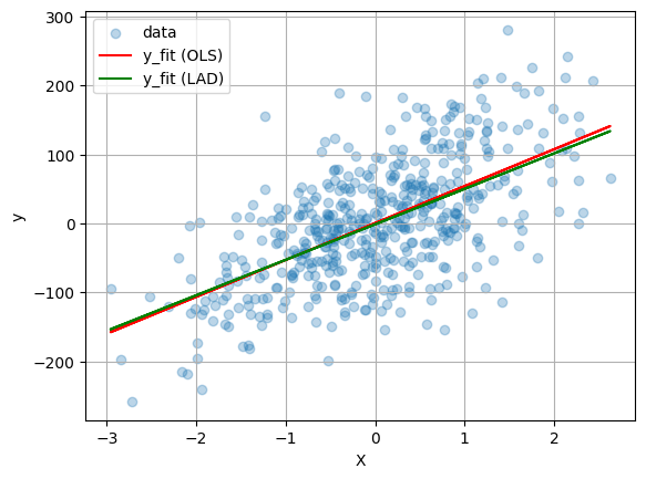
Visualizing the results and comparison with LAD regression

def lad_regression(X, y):
    m = AMPL()
    m.eval(
        """
      reset;

      set I;
      set J;
      
      var ep{I} >= 0;
      var em{I} >= 0;
      var m{J};
      var b;

      param X{I, J};
      param y{I};

      subject to residuals{i in I}:
        ep[i] - em[i] = y[i] - sum{j in J} X[i,j]*m[j] - b;

      minimize sum_of_abs_errors:
        sum{i in I} (ep[i] + em[i]);
    """
    )

    n, k = X.shape

    m.set["I"] = list(range(n))
    m.set["J"] = list(range(k))

    m.param["X"] = X
    m.param["y"] = y

    m.option["solver"] = SOLVER_LO
    m.get_output("solve;")
    return m


m = lad_regression(X, y)
m_lad = [m.var["m"][j].value() for j in m.set["J"].members()]
b_lad = m.var["b"].value()
print("\nLAD Regression\n")
print("m:", *m_lad)
print("b:", b_lad)
print("Sum of abs squares:", m.obj["sum_of_abs_errors"].value())

LAD Regression

m: 51.42857640061373
b: -1.413026812508927
Sum of abs squares: 27907.63319057619

y_fit = np.array([sum(x[j] * m_ols[j] for j in range(X.shape[1])) + b_ols for x in X])
y_fit2 = np.array([sum(x[j] * m_lad[j] for j in range(X.shape[1])) + b_lad for x in X])

if n_features == 1:
    plt.scatter(X, y, alpha=0.3, label="data")
    plt.plot(X, y_fit, "r", label="y_fit (OLS)")
    plt.plot(X, y_fit2, "g", label="y_fit (LAD)")
    plt.xlabel("X")
    plt.ylabel("y")
    plt.grid(True)
    plt.legend()

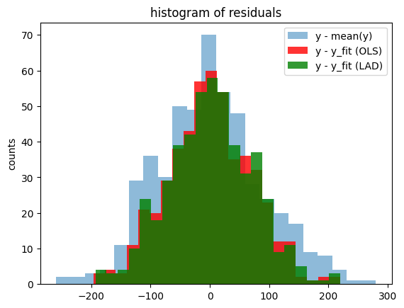
plt.figure()
plt.hist(y - np.mean(y), bins=int(np.sqrt(len(y))), alpha=0.5, label="y - mean(y)")
plt.hist(
    y - y_fit,
    bins=int(np.sqrt(len(y))),
    color="r",
    alpha=0.8,
    label="y - y_fit (OLS)",
)
plt.hist(
    y - y_fit2,
    bins=int(np.sqrt(len(y))),
    color="g",
    alpha=0.8,
    label="y - y_fit (LAD)",
)
plt.title("histogram of residuals")
plt.ylabel("counts")
plt.legend()
plt.show()